Category: Calibration & Air Adjustment

All hort articles on sprayer calibration and air adjustment.

  • Centrifugal and Diaphragm Pumps

    Centrifugal and Diaphragm Pumps

    Press Play to hear the audio version of this article

    Adjusting Sprayer Settings

    Operators are encouraged to adjust airblast sprayer settings to conform to the variability in canopy size, density, spacing, and weather conditions. The efficiency and accuracy of the application is improved through the regular and independent adjustment of travel speed, nozzle output, and air settings.

    Airblast design is highly variable.

    Inflexible sprayer design results in a suboptimal match between equipment and crop. For example, sprayers intended to blow across multiple rows in a single pass are promoted for their high productivity, but typically compromise either coverage uniformity or drift control. In another example, low volume mist blowers utilize high speed air to atomize spray and are promoted as a means for saving water and/or pesticide. But, for many such sprayers, moderating air speed to reduce drift potential causes undesired changes to spray quality.

    Even with geared fans, many of Ontario’s airblast sprayers are overpowered for vines, canes, bushberries and high-density orchards. I am uncomfortable with manually obstructing the air intake or adjusting fan blade pitch for safety reasons. Fan gears and travel speed are excellent means for adjusting air energy. Alternately, we have sometimes had success reducing air energy by gearing the tractor up and throttling down (GUTD), but it’s only for very specific situations.

    It has been my experience that centrifugal pumps on axial airblast sprayers can undermine adjustment efforts when spraying small to medium sized canopies (i.e. not tree nut or citrus). In the case of GUTD, slowing the fan reduces pressure at the nozzle. Modest pressure regulation may be possible, but typically the operator must swap to larger nozzles to maintain flow. Hollow cone nozzles are only available in large flow increments (average 0.5 gpm), and stepping-up often results in excessive flow. The operator may be able to increase travel speed to compensate, but this frustrates the original intention by affecting dwell time: air settings must now be reconsidered.

    Within this context, why do some Ontario airblast operators still choose airblast sprayers with centrifugal pumps? Let’s consider Ontario’s Georgian Bay area, which many manufacturers, distributors and mechanics refer to as “the last bastion of the centrifugal pump in Canada”.

    Remember as you read on, Ontario’s airblast crops are predominantly small to moderate sized canopies. Centrifugal pumps are a common and appropriate pump for large canopies like tree nut and citrus.

    Airblast Pumps (in Ontario)

    The Georgian Bay region of Ontario.

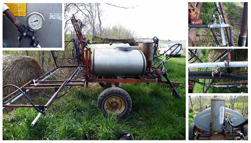
    Airblast sprayer design is highly variable, featuring a diversity of pump styles. Piston (or plunger), peristaltic, tractor-hydraulic driven centrifugal pumps are but a few. Historically, piston pumps and centrifugal pumps on John Bean and FMC sprayers were the airblast norm in Canada.

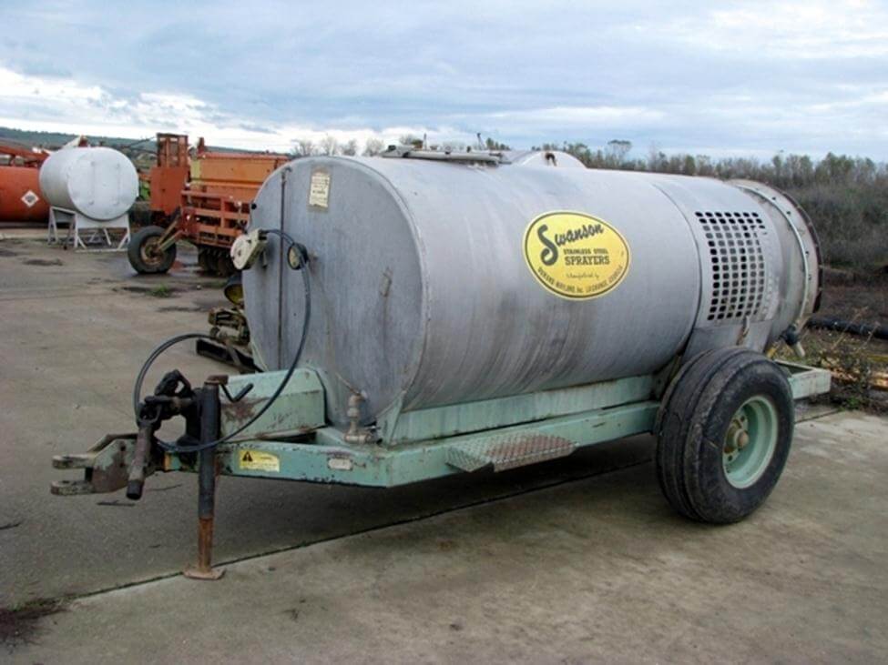
    In the 1950s, Georgian Bay was home to Swanson Sprayers (now part of DW), who manufactured airblast sprayers featuring the Myers centrifugal pump. The sprayer was a good fit for the standard apple orchards found in the region. Huge canopies required high volume applications, and the rough and craggy bark harboured mites that drove the need for drenching sprays. To achieve this, sprayers traveled at 5 km/h (3.1 mph) on 7 m (24 foot) spacing, operating at 10 bar (150 psi) to emit as much as 3,750 L/ha (400 US gal./ac). At the time, a diaphragm pump could not manage this, even traveling at 0.8 km/h (0.5 mph).

    A Swanson Sprayer (This one likely from Georgia, USA).

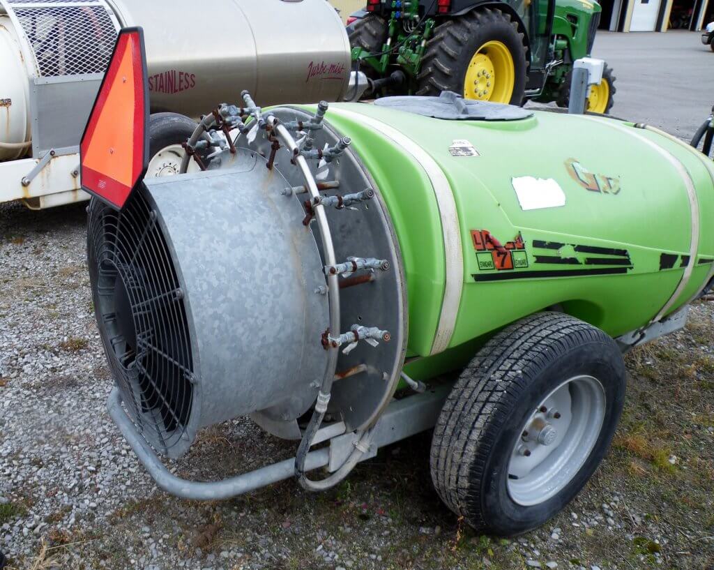
    By the 1970s Holland’s Kinkelder air-shear sprayer (centrifugal pump) was introduced to Ontario and promoted as a way to use less pesticide. Perhaps ahead of their time, they never really took off because orchards were still too large for their concentrated (i.e. low-volume) applications. By the 1980s a wave of Italian-made sprayers (e.g. the Good-Boy or GB) featuring diaphragm pumps were imported into the Niagara region by distributors such as Rittenhouse.

    Similar to the Kinkelder, this was one of Ontario’s last KWH air shear sprayers. RIP 2018.
    The Italian-made Good-Boy (or GB).

    There were many cases of misuse as unfamiliar operators failed to grease direct-drive diaphragm shafts, ran the throttle beyond 540 rpm or diverted flow intended for agitation to increase flow to the booms. Decreased agitation in relatively large tanks left concentrated spray mix to clog suction filters and destroy the diaphragm pumps. It was an inauspicious start, but the diaphragm pump rallied and today we estimate that 90% of Ontario’s airblast sprayers have diaphragm pumps, while the rest are mostly centrifugal. One Ontario airblast dealer claims to sell 50 diaphragms for every centrifugal, but not in Georgian Bay.

    Is it regional history or a long memory of diaphragm “growing pains” that propagate the demand for centrifugal pumps? Perhaps considerations of maintenance, expense or ease of use play a role. Dealers claim that the centrifugal pump is cheaper, but these savings are offset by custom installation costs. Perhaps weather conditions or the crop morphology make centrifugal a better fit? Let’s consider the relative benefits and limitations of diaphragm and centrifugal pumps.

    Design

    Centrifugal Pumps

    Centrifugal Pump – Exploded View.

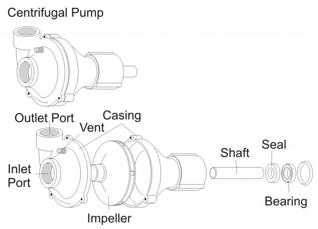
    Most centrifugal pumps prime by gravity feed which is why they are located at the bottom of the sprayer. While less common in Ontario, there are self-priming versions that reserve fluid in the case, or employ clever plumbing, permitting a more accessible location on the sprayer.

    Engine-driven centrifugal sprayers are artefacts in Ontario. The more common PTO-driven impeller operates at high speeds, requiring a >1:4 speed step-up mechanism (e.g. gearbox, pulley or hydraulic motor), and unlike diaphragms, they create smooth flow that does not require pulse suppression. While not technically required, most have a relief valve between the pump outlet and nozzle shut off valve to handle changes in pressure.

    Diaphragm Pumps

    Diaphragm Pump – Exploded View.

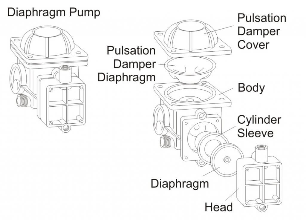
    Diaphragm pumps are self-priming and readily accessible because the shaft runs through the pump to power the fan at 540 RPM, with no need to step-up. Flow is directly proportional to pump speed which in turn depends on the tractor PTO speed. A pressure regulator is used to control bypass flow, which is convenient for making adjustments in nozzle output.
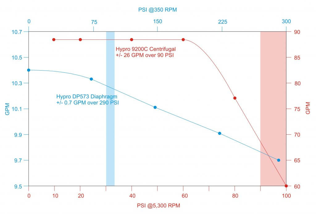
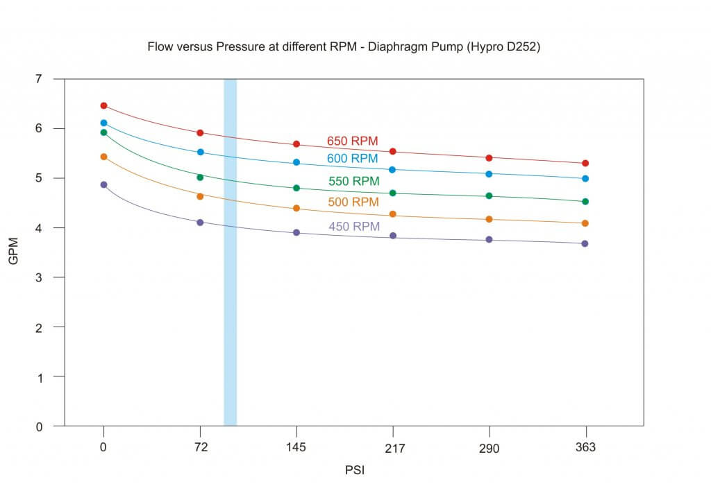
    Pump Flow and GUTD

    Centrifugal pumps are capable of higher flow at lower nozzle pressure and require more horsepower than diaphragm pumps. Note the large relative difference in flow for a centrifugal pump between the operating pressures of 90 and 100 psi (red curve shaded red) versus that of a diaphragm pump (blue curve shaded blue).
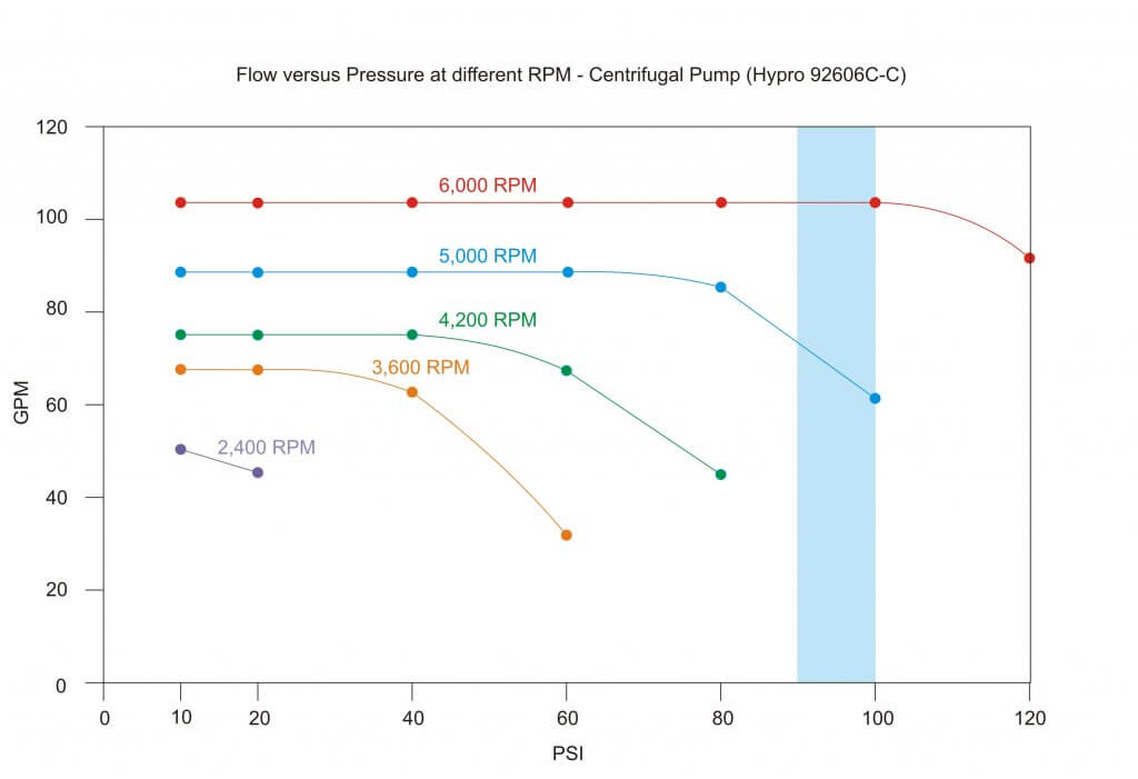
    Relative difference in flow versus PSI at constant RPM for a common Centrifugal (red) and Diaphragm (blue) pump. Shaded pressure represents 90 to 100 psi.

    Centrifugal Pumps

    The flow curve of a centrifugal pump drops off dramatically; pressure (not RPM) dictates flow. If you were to throttle back on a PTO-driven centrifugal pump, reduced flow would reduce the ability to build nozzle pressure. This means fan speed cannot be separated from nozzle pressure, and reducing air speed means re-nozzling.

    Centrifugal flow at different RPM. Shaded pressure represents 90-100 psi.

    While (unfortunately) still rare in Ontario, rate control monitors can be used (regardless of pump type) to calibrate output based on a target rate, speed and material flow using travel speed and flow sensors. Nevertheless, they cannot compensate for the aforementioned pressure loss at the nozzle if a centrifugal pump is throttled down to reduce air speed.

    In any case, throttling back on a centrifugal pump can cause a condition called suction or recirculation cavitation (aka pinging). Tiny high-pressure air bubbles form on the suction side of the impellor, explosively pitting the impellor. The damage is similar to corrosion and it causes vibration that will wear the pump prematurely.

    Any restriction on the inlet side (e.g. clogged suction strainer, collapsed/undersized line) can cause a loss of volume that can damage a centrifugal pump. “Dead-heading” (i.e. closing the outlet) is possible for a short period of time, but it quickly results in heat build-up which can cause damage.

    Diaphragm Pumps

    The flow curve of a diaphragm pump is flatter and more efficient; RPM (not pressure) dictates flow. If you slow the airblast fan by throttling the PTO below 540 rpm, flow decreases moderately, but surplus capacity allows sufficient flow to the nozzles without pressure drop. As long as the tractor does not lug, there is less noise, lower fuel consumption and therefore operator can typically adjust the air without having to change nozzles. Even if the flow changes the pressure regulator on the diaphragm pump can be used to adjust nozzle operating pressure, precluding a change in nozzle size. Convenient.

    Diaphragm flow at different RPM. Shaded pressure represents 90-100 psi.

    Diaphragm pumps are capable of high pressure, but are rarely operated above 150 psi in Ontario. Molded hollow cones (eg. TeeJet’s TXR or Albuz’s ATI) operate well in the lower psi range compared to pressure-loving disc-cores. Therefore, while regulators and springs are sized according to the pump’s maximum settings, they do not reflect the usage pattern. The relatively heavy spring is too stiff to compensate for changes in pressure (e.g. driving on hills or closing one boom) behaving more like a fixed bypass and undermining a calibration. The phenomenon is discussed more detail in this article.

    Maintenance

    Centrifugal Pumps

    A centrifugal pump with self-lubricating bearings and quality seals (e.g. carbide) that is maintained seasonally and operated in the best efficiency point of the curve will run reliably for many years.

    Proponents of the centrifugal pump claim they are low maintenance (compared to the diaphragm pump). This may be anecdotal, because of the pump’s out-of-sight position on the sprayer and their tolerance for neglect. A mistreated centrifugal pump fails by degrees, often forgotten until a seal leaks or a pressure drop is noticed. In the later situation, increased flow from nozzle wear can mask the problem as the sprayer continues to cover the same number of hectares. Often overlooked, worn or misaligned sheaves/belts on a centrifugal sprayer can also cause a loss of flow. Operators might notice a tail breeze that blows spray onto the belts can cause slippage and lower the nozzle pressure.

    Diaphragm Pumps

    Opinion is divided on the longevity and maintenance of diaphragm pumps. Some claim they are reliable and low maintenance as long as regular oil changes occur. Others suggest the complication of connecting rods, o-rings and valves require more upkeep than the simpler centrifugal. Unlike the centrifugal pump which merely loses pressure, failure on a positive displacement pump is complete and requires immediate repair

    Much depends on the diaphragm material and the products being sprayed. For example, corrosive materials (e.g. copper sulfate, urea, etc.) require polymer manifolds to minimize contact with metal. Metal manifolds do not weather well.

    The diaphragm pump can run dry for extended periods. This creates heat but does not often lead to failure. Failures occur from exposure to vacuum, which can happen with dirty suction filters or long and/or improperly sized suction lines, or even lack of oil support on the compression stroke (caused by over-revving).

    While three-cylinder designs may not require pulsation dampening, most require an accumulator to suppress the pulsing created by each stroke. Improper adjustment can lead to “hammering” that cracks mounts and valves, and can exacerbate rub-points on hoses. Diaphragm pumps that use direct drive shafts (i.e. carry the PTO to the fan) are subjected to the thrusting of the drive shaft during turns. It is important to keep them greased.

    Summarily, the longevity and maintenance requirements for either pump design seem about equal. They depend on the products being sprayed, the quality of pump materials, and adherence to the manufacturer’s instructions on correct usage and preventative maintenance.

    Conclusion

    Ontario’s airblast-specific crops have become smaller, closer and denser. High liquid volumes and air speeds are typically not required. Operators are encouraged to use Crop-Adapted Spraying to adjust fan speed and nozzle output to the crop and the weather. In my opinion, the diaphragm pump facilitates this, resulting in lowered input costs, reduced drift and improved coverage uniformity. I recognize that this requires skill and effort on the part of the operator, and setting-and-forgetting a centrifugal pump can be attractive, but it’s unacceptable if it leads to unnecessary environmental impact.

    In the end, the sprayer manufacturer chooses the pump, atomization and air-handling system while considering safety, effectiveness, reliability and price point. The operator must acknowledge the capabilities and limitations of the sprayer design when choosing the best fit for their operation.

    I still don’t know why regions like Georgian Bay seem to prefer one pump over another. Perhaps it’s simply herd mentality. Perhaps they know something I don’t. But consider: an airblast sprayer’s average lifespan is 30 years. That’s a long time to live with a decision.

    Choose wisely.

    Special thanks to the many dealers, manufacturers, engineers, mechanics and end-users that helped to inform this article.

  • Assessing Water Sensitive Paper – Part 3

    Assessing Water Sensitive Paper – Part 3

    This is the final part of our three-part article discussing methods for digitizing and processing water sensitive paper. You can read part one here and part two here.

    Morphological operations

    We can now move on to the larger shapes, or “morphology” of the objects in our binary image. Our goal is to quantify deposits by interpreting these shapes. Once again, these operations are powerful processing tools, but we must acknowledge three overriding limitations:

    1. Inconsistent stains

    Sometimes deposits do not create a consistent blue colour – they can get lighter or take on a greenish-yellow hue towards the perimeter of the stain. During thresholding, the outer edge can be accidently eroded, leaving behind an object with a jagged edge. This may lead us to underestimate the percent area actually covered. In the case of tiny stains, it might eliminate them entirely and lead us to underestimate deposit density.

    2. Overlaps

    It can be difficult to determine if an object represents a stain from a single droplet or is the result of multiple, overlapping deposits. This becomes significant when the surface of the WSP exceeds ~20% total coverage. The resulting objects may or may not have hollow centres where droplets do not overlap entirely. Misidentifying overlaps leads us to falsely conclude that an object is the result of a single, coarser droplet rather than multiple finer droplets.

    3. Ellipses

    Non-circular stains are formed when droplets scuff along the surface. Two droplets with the same volume encountering a paper at different angles can create stains with significantly different areas. We may wrongly conclude that the droplets that created them were coarser than they truly were. One approach is to use Feret’s Diameter (aka Caliper Diameter) by measuring the widest spans on the X and Y axes and taking the average. Another approach is to interpret the ellipse as a series of circular stains. Or we can decide to only acknowledge these objects when calculating percent area covered, but omit them when calculating deposit density or predicting original droplet size. Each strategy is a compromise, so it is important to be consistent and transparent when reporting results.

    Three common problems when analysing water sensitive paper.

    We’ll explore two morphological operations that can help us separate fact from fiction: Granulometry and Dilation-and-Erosion. We’re introducing these operations as part of the processing and detection step, but they may also overlap with the measurement step in our three-step process.

    Granulometry

    We can estimate the range of object sizes and get a sense of how they are distributed on the paper by filtering or “sieving” the image. Imagine pouring a mixture of sand and rocks through a series of ever-finer sieves. Doing so allows you to separate particles based on size exclusion. A granulometry function compares each object to a series of standardized objects with decreasing diameters. This isolates objects of a similar size and bins them in that size range. This is a powerful operation, but accuracy is lost when stains overlap to form larger objects. In this case, we move on to Dilation and Erosion.

    Dilation and Erosion

    Think of dilation as adding pixels to the boundary of an object. This makes tiny objects bigger, fills in any interior holes and can cause objects to merge. The number of pixel-wide dilations required to make objects contact one another can be used as a measure of deposit density.

    Erosion removes pixels from the outer (and sometimes inner) boundaries of an object. This eliminates tiny artifacts that may not actually represent stains. It can also split non-circular objects into multiple parts before shrinking them into multiple nuclei (aka centroids). These last-remaining points are not necessarily the centre of a stain, but the pixels furthest away from the original boundary.

    When a non-circular shape has more than one nucleus, they likely represent individual droplets that combined to form the larger stain. We can then use these nuclei to measure deposit density, such as in a Voronoi partition which triangulates each nucleus in relation to the two closest neighbours.

    Many image processers use both these operations sequentially. When an image is eroded and then dilated (a process called “Opening”), smaller objects are removed, leaving the area and shape of remaining objects relatively intact. Dilating and then eroding (a process called “Closing”) fills in small holes and merges smaller objects, once again leaving the area and shape of remaining objects relatively intact. We can use both of these functions to help smooth an image prior to measurement.

    (Top) Opening operations erode and then dilate the image. Moving left to right, the smaller objects tend to disappear. (Bottom) Closing operations dilate and then erode the image. Moving left to right, smaller objects either disappear or merge and holes are filled in

    Distance Transformations

    Distance transformations are advanced operations specifically used to separate objects that are densely packed. While not typically used when analyzing WSP, distance transformations are another means of identifying object nuclei. They are another means for teasing apart objects that are likely the result of overlapping deposits and then mapping their relative sizes and positions.

    Measurement

    The calculation of the area covered by deposits is straightforward. The pixels belonging to objects (the deposits) and those belonging to background are summed and then the fraction is converted to percent area covered. Research has shown that the image resolution does not significantly impact percent coverage assessments and has suggested that all image analysis software tends to produce similar results (+/- 3.5% observed when the same threshold was applied to multiple papers). This is acceptable because it’s within the variability inherent to spraying.

    We ran a similar experiment wherein we analyzed the same piece of WSP using four methods. Here are a few facts about the software we used:

    • DropScope produces images between 2,100 and 2,300 DPI. Currently, it ignores ellipses and doesn’t count anything spanning less than ~35 µm (3 pixels).
    • We set ImageJ to ignore any object spanning less than 3 pixels, which at 2,400 DPI was 30 µm in diameter.
    • We are unaware of Snapcard’s processing methods except that the software was benchmarked using ImageJ. Developers note it will underestimate the percent area covered if the image is out of focus. (Note: As of 2026, this app may no longer be supported by the GRDC).

    The images shown in the figure below were cropped from screenshots produced by each method. The actual ROI analyzed was ~3 cm2 for SnapCard, 3.68 cm2 for DropScope and 2.0 cm2 for both Epson/ImageJ methods. Our results indicate an +/- 4% difference in percent area coverage. This variability reflects the results of a 2016 journal article that compared SnapCard with ImageJ and other leading analytical software. That study claimed no statistically significant difference in percent coverage detected (standard deviations were about 20%). However, the ImageJ results tended to trend several percent higher than SnapCard. We saw this as well. And so, while resolution may not have a significant impact on percent area covered, there does appear to be some correlation.

    Percent area covered as reported by three image analysis systems. Only a minor difference was observed when resolution was doubled using the Epson/ImageJ method.

    Resolution definitely affects deposit counts. Particularly in applications that employ finer droplets. Consider the difference between detecting or missing 1,000 30 µm diameter objects. It may only amount to a fraction of a percentage of the surface covered, but +/- 1,000 objects on a 2 cm2 area is significant in terms of deposit density.

    Output

    Once a WSP image (or set of images) has been scanned, pre-processed, processed and measured, we will receive some manner of output. Some software packages create an attractive report with images, graphs and key values. These reports include percent coverage and many provide droplet density. Deposits may be binned by size, or spread factors are used to calculate the original droplet diameters and even estimate the volume applied by area. Other software packages provide raw data that can be imported into a statistical program or spreadsheet program like Excel for further analysis. Some software packages provide both.

    How far can we take this?

    Blow-by-blow data analysis is beyond the scope of this document, but how much weight should we give to coverage data obtained using WSP? The answer depends on the metric in question, but in all cases we must first acknowledge the three overriding caveats. Take it as said that they apply to everything that follows:

    1. Different brands (and even different production runs) of WSP can produce significantly different coverage metrics. When conducting experiments, use a single brand of WSP. Better still, use papers from the same production batch whenever possible.
    2. The same of piece of sprayed WSP can produce significantly different results depending on the software and protocol used to analyze it. When conducting experiments, use the same software and assessment protocol and be transparent about the process when communicating results.
    3. WSP coverage may not reflect the coverage achieved on an actual plant tissue surface. It is suitable as a relative index (I.e. papers can be compared to papers, but not to tissues) but the spread factor changes with surface wettability and the surface tension of the liquid sprayed. Note the differences in percent area covered in the following experiment with an organosilicone super-spreader:
    Difference in deposit spread on water sensitive paper versus a leaf surface using an organosilicone super-spreader and UV dye. The same volume was applied in each case and while the area increased two-fold on WSP it increased ~10-fold on an actual leaf. Image reproduced from work by Robyn Gaskin, Plant Protection Products, New Zealand.

    Recall that we started this document by listing the four pieces of information commonly sought using WSP. They were listed in order of reliability, and now we can explain why.

    • The percent surface area covered: We have established that this is the most reliable piece of data. Droplets do not spread on WSP the way they do on plant surfaces, so it will underestimate actual coverage. The results vary by analytical method, but it’s likely not dependent on resolution and still falls within the variability inherent to spraying. This metric gives us valuable and actionable information. We can say whether or not we hit a target, and evaluate whether a sprayer change resulted in more or less deposit.
    • The density of deposits on the target area: We have established that that there are limits to the reliability of this metric. It is affected by the analytical method used and can be greatly underestimated when resolution is poor or when deposits overlap in high numbers. Also, it will never reliably reflect deposits under 30 µm. Nevertheless, under controlled conditions this information does have value and is of great interest in enquiries about drift and contact fungicides.
    • The size of the droplets that left the stains: This metric is highly questionable except under controlled conditions. The many assumptions about surface tension, droplet speed, and droplet evaporation make it impossible to make definitive statements about spray quality. Finer droplets are greatly underestimated in this equation. Therefore, while there may be some value in using WSP as a relative index, this metric is a crude indication at best.
    • The dose applied to the target surface: This metric has not been discussed up to this point, but is quickly and easily dismissed. Let’s assume that a droplet with a high concentration of an active ingredient will leave a stain that is the same area as another droplet with a lower concentration. This will lead some to suggest that as long as the original concentration is known, we can back-calculate the dose (which is the amount of active on a given area). However, one droplet has the same volume as eight droplets that are half it’s diameter. This cubic relationship means that if they all deposit, the larger droplet will cover roughly 1/2 the surface area as the eight smaller droplets. Therefore, the smaller droplets spread the same amount of active over a greater area. Spread factor muddies this a bit, but ultimately it means that dose cannot be estimated from area covered. Dose is better assessed using collectors that permit the residue to be removed, such as Petri dishes, Mylar sheets, pipe cleaners, alpha cellulose cards, or glass slides.

    And so, the image analysis process described here is powerful and effective when used with water sensitive paper as long as the limitations are acknowledged. The same process can also be used with dyes and specialized collectors such as Kromekote to permit even greater resolution. But that’s another story.

    References (Further reading)

    Bankhead, P. 2014. Analyzing fluorescence microscopy images with ImageJ.

    Cunha, J.P.A.R., Farnese, A.C., Olivet, J.J. 2013. Computer programs for analysis of droplets sprayed on water sensitive papers. Planta Daninha, Viçosa-MG. 31(3): 715-720.

    Ferguson, J.C., Chechetto, R.G., O’Donnell, C.C., Fritz, B.K., Hoffmann, W.C., Coleman, C.E., Chauhan, B.S., Adkins, S.W. Kruger, G.R., Hewitt, A.J. 2016. Assessing a novel smartphone application – SnapCard, compared to five imaging systems to quantify droplet deposition on artificial collectors. Computers and Electronics in Agriculture. 128: 193-198.

    Ledebuhr, M. 2016. Small Drop Sprays.

    Marçal, A.R.S., Cunha, M. 2008. Image processing of artificial targets for automatic evaluation of spray targets. Trans. of the ASABE. 51(3): 811-821.

    Moor, A., Langenakens, J., Vereecke, E., Jaeken, P., Lootens, P., Vandecasteele, P. 2000. Image analysis of water sensitive paper as a tool for the evaluation of spray distribution of orchard sprayers. Aspects of Applied Biology. 57.

    Panneton, B. 2002. Image analysis of water‐sensitive cards for spray coverage experiments. Applied Eng. in Agric. 18(2): 179‐182.

    Salyani, M., Zhu, H., Sweeb, R.D., Pai, N. 2013. Assessment of spray distribution with water-sensitive paper. Agric. Eng. Int.: CIGR Journal. 15(2): 101-111.

    SnapCard website. University of Western Australia and the Department of Primary Industries and Regional Development, Western Australia. (Note: As of 2026, may no longer exist).

    Syngenta. 2002. Water‐sensitive paper for monitoring spray distributions. CH‐4002. Basle, Switzerland: Syngenta Crop Protection.

    Turner, C.R., Huntington, K.A. 1970. The use of a water sensitive dye for the detection and assessment of small spray droplets. J. Agric. Eng. Res. 15: 385-387.

  • Greenhouse Foggers

    Greenhouse Foggers

    Greenhouse application equipment spans from the humble squirt bottle, to gas-powered foggers, to robots equipped with hydraulic vertical booms. The variety of spray equipment available reflects a variety of needs, just as a carpenter’s toolbox contains different tools designed to do different things. In order to get the most out of foggers and misters, it’s important to understand how they differ from “conventional” hydraulic spraying.

    A greenhouse robotic vertical boom sprayer.
    A greenhouse robotic vertical boom or “tree” sprayer

    Mechanical and Chemical Spread

    For many greenhouses, water is the carrier that dilutes and delivers the chemistry to the target. Water has a high surface tension and tends to bead on target surfaces. Dr. Heping Zhu (USDA, Ohio) created some amazing videos using controlled water droplets and both waxy and hairy leaves. In first video we see how water beads up on a waxy leaf, and as it evaporates, the area touching the leaf surface remains small. In the second, we see the droplet get hung up on a trichome (leaf hair) and evaporate while suspended above the leaf surface.

    Neither situation is desirable since the goal of spraying is to maximize the level of contact between droplet and target. Contact can be increased via mechanical spread or chemical spread (see figure below).

    The degree of chemical spread can be increased by adding adjuvants such as non-ionic surfactants to reduce surface tension. In the videos below we see the same controlled droplets with the same volume of liquid, but they now include a non-ionic surfactant. In the first video we see a greater degree of contact with the waxy target surface as the droplet spreads. In the second, the droplet does not get caught by the trichome, but splashes down onto the surface. Some product labels advise the inclusion of adjuvants and others are already formulated with them. In the case of surfactants, be aware of the potential for run-off and phytotoxicity.

    Mechanical spread requires us to break a single, larger droplet into several smaller volumes to increase the degree of contact. This approach usually comes with a caveat about evaporation, but this is rarely a concern in a humid greenhouse. As for the risk of drift, once again, in greenhouses it is a different story than conventional spraying. Spray drift is desirable! Lateral air movement is very important to encourage plant canopy penetration and prevent droplets from merely settling on upward-facing plant surfaces. While some equipment generates its own air, the air currents in the greenhouse are often the primary means for suspended droplets to circulate throughout the space. In either case, air could be considered the carrier instead of water. Too little air flow, or gaps in circulation, will reduce coverage. Too much air flow (specifically, greenhouse air circulation) may cause plants to exhibit stunting.

    Spray Quality (ISO)

    Here’s how ISO/DIS (5681:2019 Equipment for crop protection — Vocabulary 3.2.1) defines the spray quality produced by misters and foggers:

    • (3.2.1.13) MIST: “Spray with volume median diameter between 50 µm and 100 µm.”
    • (3.2.1.14) FOG: “Aerosol spray with volume median diameter under 50 µm where the droplets are effectively suspended in air with little or no settling by gravity.”

    These droplets do not behave like coarser droplets. For more information on droplet movement, survivability, and transfer efficiency, download Purdue Extension’s “Adjuvants and the Power of the Spray Droplet”.

    Water sensitive paper has limited utility when diagnosing coverage from foggers. Sophisticated optical scanners may be able to detect deposits as small as 25 µm, but this is open to debate. Manufacturers do not support the use of papers when quantifying deposits less than 50 µm , and some draw the line at 100 µm.

    In the following image, papers were used to diagnose coverage (from clean water) in a poinsettia greenhouse. The two papers on the right were located in the canopy and sprayed using a thermal pulse fogger and a hardware store style hand pump. The paper on the left was held directly in the path of the fogger while using the smallest nozzle provided with the unit. The spray enveloped the paper (and the person holding it). Close inspection showed tiny deposits, and the SnapCard app detected 4.5% coverage, but this greatly underestimates the actual deposition and does not account for the droplet count.

    UV dyes are the preferred method for analyzing coverage from foggers.

    Fogging and Misting Equipment

    Greenhouse spray equipment can be classified by droplet size, but also by the spray volume they employ.

    High Volume (HV)

    These applications are performed at pressures ranging from 500 to 4,285 kPa (75 to 700 psi) employing flow rates of 3.9 to 5.7 L/min (1 to 1.5 US g/min). They use standard label rates to accomplish a dilute application by broadcasting droplets larger than 100 microns. The goal is to cover all surfaces without incurring run-off. Examples of HV application equipment include backpack sprayers, trailed sprayers and boom sprayers. Practice and self-calibration are necessary to achieve the desired results when using manual HV sprayers.

    Targeted Low Volume (LV)

    These applications are performed at high pressures around 20,685 kPa (3,000 psi) employing flow rates approaching 1 L/min (0.26 US g/min), covering 93 m2 (1,000 ft2). They apply reduced rates over a given area and create droplets between 25 and 100 µm. These are concentrated sprays that do not result in wet foliage. LV applications are particularly good in high-humidity environments, when it is desirable to minimize the moisture on leaves. Examples of LV application equipment include aerosol cans.

    Ultra-Low Volume (ULV)

    These applications employ flow rates approaching 2 L/min (0.52 US g/min), covering 930 m2 (10,000 ft2). They require concentrated solutions, but apply reduced rates per area using droplets less than 25 µm. ULV applications will not raise greenhouse humidity and are a good choice when days are short and nights are long. They are also an excellent way to apply disinfectants for complete space sanitation before starting a new crop. It is important to ensure vents are closed and fans are off during sanitation. Examples of ULV application equipment include total release cans, auto foggers and thermal pulse foggers.

    PulsFOG hand-held ULV cold fogger

    Thermal pulse foggers are unlike other ULV equipment and warrant special consideration. The design of the pulse fogger has remained virtually unchanged since the 1940’s. Smaller, 24 hp machines are used in smaller operations but range up to large 175 hp machines. Tank size ranges from 10 to 50 L, where 10 L should be enough to cover 4,645 m2 (50,000 ft2) in about 10 minutes, depending on crop density. Their range is about 35 m (115 ft) from the point of release.

    Thermal Pulse foggers do not create aerosol using air shear – they use combustion (80 to 100 explosions per second) to shatter spray into a fog and propel it via positive pressure. Heat is a by-product of the engine, making it an unsuitable method for applying biological products.

    However, water-cooled foggers such as Dramm’s Bio Pulse Fogger reduce the exhaust temperature below 100 °C to make the application bio-rational. This has the added advantage of making droplet sizes more consistent and preventing spray from evaporating too quickly before it diffuses to the target.

    Dramm Bio Pulse Fogger.
    Dramm Bio Pulse Fogger

    Using a Fogger

    Dramm recommends that operators use approximately 1 L of carrier in 5 L of spray mix, but a higher proportion of carrier would be required for more viscous products. Start with a full tank of clean, high grade gasoline and once the fogger has been started, run it continuously until the application is complete. Leave it running even when moving between Quonset huts (see below).

    Know when to use a pulse fogger versus an auto fogger. Auto foggers are convenient because the operator can set them and leave. However, in the case of multiple huts, it is more efficient and timely to use a thermal pulse fogger.
    Know when to use a pulse fogger versus an auto fogger. Auto foggers are convenient because the operator can set them and leave. However, in the case of multiple huts, it is more efficient and timely to use a thermal pulse fogger.

    Do not leave the manual fogger running unsupervised as an auto fogger: If they stay stationary, or aim directly at the canopy (as in hydraulic spraying), they could drench and potentially damage nearby plants.

    When fogging, aim between the plants, such as the alleys and between hanging plants. This allows the fog to expand and permeate canopies for the best coverage. When spraying is done, be sure to release the pressure created in the spray tank to prevent accidental back flow into the gasoline tank.

    And, because it’s convenient to include the math in this article, here are the formulae for calculating greenhouse volume to help you determine rates.

    Care and Maintenance

    HV, LV and ULV equipment requires model-specific cleaning and maintenance, according to manufacturer’s instructions. Even when sprayers are kept in prime condition, they are only as good as the operator’s understanding. When the wrong product is applied by the wrong machine using the wrong method, operators risk poor control, crop damage and increased potential for pesticide resistance. For more information, read the instructions that came with your sprayer, or contact the manufacturer.

    Thanks to Louis Damm and Dr. Heping Zhu for their contributions to this article.

  • Crop-Adapted Spraying (CAS) and an Apple Orchard Case Study

    Crop-Adapted Spraying (CAS) and an Apple Orchard Case Study

    An orchard spraying scenario

    Here’s a common situation: An orchardist following IPM identifies a pest that poses an economic threat. It’s an annual pest and spraying is really a matter of when, not if. The operation is 150 acres and runs three airblast sprayers; two have a tower and one does not. Multiple varieties are planted in several blocks on different rootstocks and they are at different stages of maturity. The newer blocks are trellised high density trees and the older blocks are semi-dwarfs on different row spacing. Let’s also imagine the pruning team hasn’t finished yet, so some trees are not pruned.

    The orchardist turns to the pesticide label to decide how to spray such variable targets. It prescribes a range of doses per planted area (not canopy size), depending on the pest pressure. It advises the orchardist to use “enough water” to ensure “good coverage” without incurring “runoff”.

    The orchardist recognizes that the label is vague, and elects to rely on what has worked historically: A water-soluble pouch is dropped into each tank (dose is close enough), and each sprayer operator is instructed to drive at an efficient speed (get it done because rain is coming), spraying until the tank is empty. They say that if a tank is running low before the job is done, speed up and stretch it. If the spray is overshooting a younger planting, they suggest turning off the top nozzles and/or driving faster.

    Airblast operators face this situation regularly. The question is: “Is there a problem with spraying this way if it results in a respectable crop of quality fruit?” Agricultural engineers specializing in application technology in Spain, Australia, Great Britain and the United States say there is a problem, and on behalf of Canada, I completely agree with them.

    Canopy and Sprayer Variability

    The fundamental problem is inconsistent spray coverage and avoidable waste (of time, water and pesticide) due to variability. Our scenario notes multiple sprayer operators, different models of sprayer, and a range of varieties, orchard architectures and canopy management practices. The label does not allow for any of these factors, adhering to a rate based on planted area and remaining silent on water volume.

    International peer-reviewed journal articles stretching back to the sixties have conclusively demonstrated order-of-magnitude differences in the area-density of orchard canopies from one acre to the next. There can even be fold-differences in canopy area-density in the same planting as the season progresses. A label prescribing a fixed dose based on the area planted is not appropriate for any vine, bush, cane or tree crop, and the result is that more crops are over- or under-sprayed than receive appropriate coverage.

    Let us not forget the variability that comes from a poorly adjusted sprayer. I won’t to attempt to quantify the impact (although some researchers have suggested order-of-magnitude differences from sprayer to sprayer). Instead, let’s illustrate it as a conceptual “before and after”:

    Before: Potential spray loss and inconsistency before adjusting sprayer to match the canopy
    After: Coverage variability reduced and unnecessary waste mostly eliminated.

    Beyond the immediate impact on efficiency, variability makes it difficult to diagnose pesticide effectiveness. As an example, there was a scab outbreak in Ontario in 2009 that elicited questions about timing, weather, product choice and resistance. There was very little attention given to spray coverage, which to my mind should have been the first question if only to eliminate it as a potential culprit. This is because each operation interprets labels differently, and very few confirm coverage in any quantifiable way. This practice makes it more difficult to identify a cause when crop protection fails.

    Optimizing pesticide rates

    That was a lot of preamble to describe an issue that many orchardists are already aware of. What is needed is a way to adjust the amount of pesticide per unit ground area (i.e. the label’s prescription) to achieve consistent foliar coverage for canopies of varying shape and density. The concept is visualized in the following figure. In addition, the method has to be simple, intuitive and effective.

    Many models have been proposed to tackle the dose expression issue, including Tree-Row Volume, Leaf Area Index, Leaf Wall Area, PACE+ and DOSAVIÑA. There are advantages and disadvantages to each method. Standing on the shoulders of giants, we combined aspects of each of these models, including incorporating coverage factor research from USDA ARS work in nurseries, to develop the Crop-Adapted Spraying (CAS) method. It is neither complicated nor sophisticated. It formalizes a series of qualitative calibration techniques and the objective is to achieve a target foliar coverage pattern. When achieved with sufficient accuracy, pesticide efficacy is maintained and waste is greatly reduced.

    Caveats

    Perhaps I shouldn’t point out flaws before I describe the model’s effectiveness, but it’s important to understand that CAS relies on a few critical assumptions.

    The first assumption is that the sprayer operator’s typical ratio of formulated product to carrier is appropriate. We need a starting point for adjusting the amount of pesticide per unit planted area, and unless the label specifies a concentration (i.e. a ratio of formulated product to water) or a minimum amount of product per planted area, this is a reasonable starting point. The appropriateness of this assumption is evidenced by a history of satisfactory pest control in the orchard.

    The second assumption lies in defining a threshold for sufficient coverage, and this is a real challenge. Applications can be concentrate or dilute. Some products translocate in the leaf or redistribute on the leaf surface while others do not. Even the droplet size employed (e.g. A mist blower’s fines compared to Medium-Coarse droplets produced by an air induction nozzle) will affect dose, bioavailability and how long residues are active. So, how does one draw a universal line in the sand and say “this much is enough”?

    Our threshold for suitable foliar coverage has evolved through experience, literature review and independent experimentation in several countries and in multiple 3D cropping systems. We propose 10-15 % surface coverage and a minimum of 85 droplets per cm2on a minimum 80% of the canopy. This standard is intended to be practical, versatile and robust in order to safely represent sufficient coverage for most foliar insecticides and fungicides. It is not suitable for ultra-low volume sprayers (e.g. misters, foggers, air-shear), nor is it intended to be a rigorous, scientific absolute.

    For example, a drench application, such as streptomycin or dormant oils, will obviously require more coverage. Plant growth regulators like thinners, stop-drops and foliar nutrients have their own unique criteria. Products that work through vapour redistribution (e.g. some forms of sulfur) and bio-rational products have a minimal dose threshold that must be ensured per planted area, no matter the water volume used. In these cases, Crop-Adapted Spraying may not be appropriate.

    So while it is the nature of models that they may not hold in every situation, this threshold has proved successful in multiple Ontario apple (later in this article) and highbush blueberry operations.

    The method

    The method is a simple and iterative approach that allows growers to adjust the product rate and sprayer output in relation to canopy and sprayer effects on deposits. Follow these steps to adjust the sprayer and optimize coverage. Only do so in conditions you would normally spray in.

    Step 1

    The sprayer should receive all seasonal maintenance prior to first use and undergo a visual inspection before each spray day.

    Step 2

    Park the sprayer in an alley between rows of trees and tie 25 cm (10 in) lengths of ribbon along the air outlet. That would be the deflectors on a low profile axial sprayer, the hubs of multifan systems or the ducted outlets on towers. Turn on the air and extrapolate where the air is aimed. Adjust the air to just overshoot the top of the canopy.

    Step 3

    It is important that the spray slightly overshoot the canopy height. It is less important to spray the lowest point of the canopy as secondary deposition tends to provide sufficient coverage. This may change if fruit weighs down the branches. Ensuring a full swath, turn off any nozzles that are not required. For small and medium canopy sizes, consider using air-induction hollow cones in the top positions of each boom to reduce drift. You may have to increase the rate in those positions to compensate for the fact that nozzles producing larger droplets produce fewer droplets.

    Step 4

    Affix 25 cm (10 in) ribbons to the upwind and far side of one or more trees. At minimum, affix them at the treetop and along the widest portion of the canopy. With the tank half-full of water, drive past in the spraying gear at the ideal RPMs with the air on. A partner in the next alley should see the highest ribbon move. Ideally the other ribbons will waft as well, but in large, dense canopies they may not. In this case, ensure leaves are moving beyond the trunk. No ribbons should strain straight-out.

    This will determine if more/less air is required from the airblast sprayer. The operator can change fan speed (e.g. fan gear), or adjust the sprayer’s travel speed. Lower speed causes air to go higher and deeper and vice versa. In some cases, operators can reduce fan speed by reducing the tractor PTO revolutions by gearing up and throttling down. When air is corrected, determine ground speed in the orchard using smartphone GPS app or a calibration formula.

    Step 5

    Place and interpret water-sensitive papers per this article. If coverage is excessive, reduce output in corresponding nozzle positions (by replacing them with lower rate nozzles). If you see less than ideal coverage, increase the nozzle rates in those positions.

    Be aware that excessive coverage may be unavoidable in the outer edge of the canopy, given that spray must pass through to get to the centre. It is not unusual to see half the deposition mid-canopy when the outside is saturated. Also be aware that ambient wind speed and humidity have significant impacts on coverage. Therefore, only test coverage in conditions similar to your typical spraying conditions.

    Step 6

    When the canopy grows and fills in sufficiently (usually after petal fall), you may have to reassess coverage to reflect a larger, denser canopy with more surface area. Given the critical nature of early season fungicide applications, it may be preferable to have slightly excessive coverage early season and allowing it to self-correct as the season proceeds. If you are suspicious that the spray is being stretched too thin or you are unsatisfied with the coverage, increase the output.

    For high density trees, there may be no need to increase output mid-season. Early in the season, wind travels relatively unimpeded in a high-density orchard and will blow spray off course, reducing coverage and requiring higher water volumes or possibly more air to compensate. As the trees fill in, the average wind speed is reduced and more spray can impact on the target.

    Mixing and Work Rate

    When the correct sprayer settings and volumes have been determined, the operator will mix their spray tank as they would for their typical application. The sprayer will likely cover more orchard than it has in the past, and the operator will have to re-assess how many tanks are required pre and post petal-fall. If your sprayer is employs conventional hydraulic nozzles (that is, it is not a low-volume sprayer), it is not advisable to go below 400 L/ha (~40 gpa).

    This is where OrchardMAX (the free CAS calculator app) can help the operator ballpark the correct rates for each nozzle position and estimate work rate, tanks required, and any potential savings in product.

    Yes. There’s an app for that.

    Apple Orchard Case Study

    Three Ontario apple orchards (and one Nova Scotia orchard) agreed to test the model. A block of trees was randomly selected from each operation to serve as the treatment condition. These trees received spray according to the CAS model. The rest of the orchard was sprayed according to the grower’s traditional methods. The orchards included several varieties and represented both semi-dwarf and high density plantings.

    OrchardTypical spray volume (Control)CAS spray volume (Treatment)% SavingsVarieties (age)Orchard StructureYears in study
    Orchard 1486 L/ha373 L/ha23%Gala + g. Del (~10 yr old)High density3
    Orchard 2748 L/ha478 L/ha &

    608 L/ha = 543 L/ha

    28%Macs + Empires (~30 yr old)Semi-dwarf3+
    Orchard 3577 L/ha

    (660 L/ha)

    407 L/ha39%

    (38%)

    Gala + Fuji (~20 yr old)High density2
    Nova Scotia544 L/ha416 L/ha33%Jonogold (~10 yr old)High density1+

    According to the model, each grower sprayed anywhere from 20-35% less per hectare in the CAS block than in their traditionally-sprayed block. In many cases, the overall canopy coverage was improved in the CAS block compared to the traditional method simply by aiming formally wasted spray into the canopy, and reducing volume in those areas that were unnecessarily drenched.

    A scout was dispatched to monitor insect and disease activity each week for ~15 weeks. They observed a typical IPM scouting protocol and were not informed which block was the traditional control and which was CAS treatment. Data was transformed where appropriate for analysis of variance. In almost every case, there was no significant difference in counts between the CAS treatment and the grower’s traditionally-sprayed control (p=0.05). In those few cases where a pest had higher counts in the CAS block, the counts were so far below a spray threshold as to be insignificant.

    If we look more closely at the three (of 128) ANOVA comparisons of control to treatment, we see that economic thresholds are rarely an issue, and essentially, difference between control and treatment are moot.

    2015_TSSM_O1_Y2
    2015_ERM_O1_Y3
    2015_ERM_O1_Y2

    This study was repeated over three years. Having examined the data to determine if three years of optimized doses had any effect on pest populations, results suggest no such effect.

    Apples were randomly sampled for destructive analysis at harvest and the total counts of any and all damage are shown below. This is simply a tally, and no statistical significance is implied. Note that Orchard 3 was only involved in the study for two years, and unfortunately a killing frost destroyed their harvest in their second year, so we didn’t have much to harvest.

    Apple_data_3_years

    An important part of knowledge transfer is whether or not growers will choose to adopt a method once the instructor is gone. By year two the biggest challenge was ensuring the orchardists in the study continued to spray the control block at their traditional volumes! They were more than willing to adopt the method wholesale and all three did so starting in 2016. Further, colleagues in Nova Scotia performed their own CAS trial for two years, and reported no significant difference in pest activity or apple quality. They accomplished this simply by following a written protocol.

    The orchardist’s enthusiasm, the ability for the study to be replicated without my direct involvement, and the successful results speak to the viability of the method.

    We would like to thank the researchers that developed the methods CAS is based upon, statistician Behrouz Eshani, the orchards that cooperated in the study, my OMAFRA colleagues and the OMAFRA summer students that scouted those orchards for three years.

    More information

    This method of application is really no more sophisticated than the pro rata practice of turning off nozzles that are aiming at the ground or above the target. It will take time for operators to get comfortable with the new volumes (and potentially reduced dosage) and regular scouting is highly encouraged to confirm they are achieving control.

    The maintenance, calibration and operation of an airblast sprayer is an involved process. Collectively, the sprayer setup, weather and crop morphology all influence the coverage obtained from an application. A fundamental understanding of application technology is required before attempting to optimize dosage using the CAS method. We suggest grabbing a copy of the second edition of Airblast101 – Your Guide to Effective and Efficient Spraying. The digital version is a free download, but you can buy a hardcopy as well.

    Finally, take a few minutes to watch this video by AAMS-Salvarani. In many European countries such as Belgium , France and Germany, sprayers must be calibrated regularly. While there is no mention of air speed adjustments, many of the steps in this video correspond with the airblast adjustments relating to Crop-Adapted Spraying.

  • Compulsory, Standardized Sprayer Inspections

    Compulsory, Standardized Sprayer Inspections

    Spring always brings renewed interest in sprayer calibration. This is good, because a well-maintained and calibrated sprayer will protect crops more effectively and efficiently, as well as reduce the potential for off-target drift and point source contamination.

    Presently, there is no nationally-recognized standard for sprayer calibration in either Canada or the United States. As a result there are many methods, some more stringent than others, spanning activities relating to seasonal maintenance through to precise diagnostic measurements. This means an operator can be in compliance with programs such as CanadaGAP (a food safety traceability standard for fruit and vegetables), and yet only perform the most rudimentary adjustments.

    I was first made aware of “compulsory inspections” in 2009 when I started noticing certification stickers on certain European import airblast sprayers. Some Ontario tender fruit and grape growers familiar with the European standards asked why we didn’t enforce standardized calibration program as they do in Europe. I was surprised to hear a farmer ask for more paperwork, so it made me wonder, are Canada and the US overdue for a change?

    All sprayers, from large, commercial field and airblast sprayers, to the more humble home-grown sprayers (see below) benefit from regular servicing and calibration. And yet, sprayer calibration in Canada and the US remains largely voluntary and highly variable depending on the size of the operation, sprayer design and the willingness/skill of the operator.

    Canada and the US: Then

    In the mid 1980’s, University of Nebraska engineers and Successful Farming Magazine published a study showing that un-calibrated spray applications were costing US farmers ~$1,000,000,000 per year. The article was infamously called “The Billion Dollar Blunder”. You can download the original journal article describing the survey here.  It was estimated that fewer than 5% of applications were within 5% of the desired rates. Spray overlaps and poor calibration resulted in over-applications of more than 20%.

    At the time it was eye-opening and received a lot of attention. In 2006 the original study was revisited (see here), and even with advances in precision application, there was a disappointing lack of improvement. Bill Casady, University of Missouri Extension agricultural engineer, estimated that if 20 minutes of calibration can save 5% on 500 acres in an application sprayed at $25/ac ($61.75/ha), then the 20 minutes of effort worked out to $1,875 / hour. Now that’s a solid return on investment!

    Belgium: Then

    Belgium recognized and addressed this issue more than twenty years ago. In 1995, following the lead of the Netherlands and Germany, Belgium’s Ministry of Agriculture mandated that all spraying equipment (save backpacks) be inspected every three years. At the time, other countries such as Sweden, Hungary and Austria had similar, albeit voluntary, programs.

    Belgian farmers received letters asking them to make their sprayers available for testing by a Ministry-appointed institution, in locations no more than 10 kilometers from their operations. The institution’s trained technicians would subject the sprayers to a regimented, standardized inspection. When the equipment met the standard, they would receive a permit in the form of a sticker (see below) attached to the sprayer. The growers paid for this service, based in part on the size of the sprayer.

    In order to introduce the process to the Belgian farmer, a short documentary was produced. If you would rather not watch the preamble explaining why the prudent use of chemistry is critical to agriculture, and get right to the sprayer inspection process, skip ahead to 3:35.

    What follows is a brief outline of that 1995 process, which I’m told is similar to the process currently used in Belgium:

    1. Administrators perform visual checks to assess the general condition of the sprayer (e.g. obvious maintenance, safety and operational issues).
    2. Boom balance (where applicable), hinges, boom ends and boom sturdiness is checked.
    3. Nozzle spacing and orientation of nozzle bodies is inspected.
    4. All points of filtration are inspected.
    5. For boom sprayers, a spray pattern distribution used to be performed, but it wasn’t diagnostic enough. Instead, a pressure gauge / nozzle combo is used in each position to check for pressure fluctuation, and to ensure each tip had a flow rate within 5% of the average and no more than 10% deviation from the manufacturer’s rate.
    6. For airblast sprayers, the overall output of the sprayer is measured to determine nozzle wear using individual collectors clamped onto each position.
    7. For sprayers with rate controllers, calibrated collection bags are attached to a few nozzles and the sprayer drives a 100 metre course while spraying. The actual output is compared to the expected.
    8. Finally, the farmer receives a report outlining issues that need to be remedied before the sprayer is certified.

    SPISE: Today

    Today, collaborating European countries are members of SPISEStandardized Procedure for the Inspection of Sprayers in Europe. Established in 2004 by founding members from Belgium, France, Germany, Italy and the Netherlands, the SPISE Working Group aims to “further the harmonization and mutual acceptance of equipment inspections”. They also work to continually improve the inspection / calibration process.

    Their website hosts a number of sprayer-related resources, but the SPICE Advice handbooks are perhaps most valuable to the sprayer operator. Click either image below to download them as PDF for airblast or field sprayers:

    This more current video by AAMS-Salvarani goes though the inspection and adjustment process for airblast sprayers. While there is no mention of air speed adjustments, many of the steps in this video correspond with the airblast adjustments relating to Crop-Adapted Spraying which has proven very successful in Canada.

    Canada and the US: Tomorrow

    Regular, third-party mediated inspections offer many potential benefits to the average operator. But, in order to realize gains in crop protection and environmental stewardship, perhaps there are two programs required: One to certify the sprayer and the other to certify the sprayer operator.

    1. A sprayer inspection program would focus on sprayer maintenance rather than calibration. Maintenance occurs at regular intervals to ensure spray equipment is operating optimally. Calibration is an ongoing process intended to match the sprayer to the conditions in which it’s operating, and that requires an educated sprayer operator.
    2. Sprayer operator education programs such as Ontario’s Grower Pesticide Safety Course, or Penn State’s Pesticide Applicator Certification Course already exist, but they are not offered in every state or province, and they are often voluntary or perhaps specific to a particular expertise (e.g. not applying to custom applicators or airblast operators).

    They could start as voluntary, pay-for-service pilot programs to see if operators appreciate how much better their sprayers are functioning, and to quantify how much waste is been reduced. They wouldn’t necessarily have to be government-run; Industry or Academia may be better conduits. So, what would be required to develop and implement these two programs?

    • We would need to agree on a robust and generic sprayer inspection protocol. We have several European examples to draw on.
    • We would need to agree on the minimal content for a sprayer operator course. Again, we have many to draw on, with the obvious understanding that the core curriculum would be amended to reflect various state and provincial requirements.
    • We would need a trained, third-party organization to take responsibility for overseeing and implementing the two programs.
    • And, of course, we would need the funds to initiate both programs before they would eventually become self-sustaining.

    So, are we dreaming in Technicolor? If responses to this article are any indication, there are those in western society that lash out at the idea of mandatory requirements. But there are supporters, too. Maybe we can learn from those European countries that have been doing this for more than 20 years.

    Thanks to Jan Langenakens of aams for reviewing this article, and providing the videos.